Overview

The Wetlands Explorer tool integrates a variety of spatial data layers—including study area boundaries, species at risk, critical habitat, protected areas, freshwater features, and surface water dynamics—to support environmental assessment, planning, and conservation in the Thompson-Okanagan region. It features high-resolution wetland predictions derived from a Random Forest classification model, using Sentinel imagery, topographic data, and LiDAR where available. Outputs include 3m and 18m resolution maps for the Okanagan and Thompson-Nicola areas, respectively, along with associated wetland probability layers.

To account for differences in data availability, two separate models were developed: one for the Okanagan, incorporating LiDAR-derived terrain data, and one for the remainder of the study area using the Canadian Digital Elevation Model. Both models were trained using existing wetland data (e.g. Freshwater Atlas) and a broad set of environmental variables, including vegetation and moisture indices, topographic features, and proximity to streams. The resulting maps reveal patterns of wetland distribution and hydrologic connectivity that support informed decision-making, with field validation recommended for site-specific applications.

Technical Details for the Random Forest Wetland Predictive Models – Thompson and Okanagan Regions

Written by Kristina Deenik, MSc, RPBio & Evan Lavine, BES, ADGIS
2025-05-30
Model outputs are accessible through the Thompson-Okanagan Wetland Explorer Tool. Please contact us or refer to the main tool documentation for access details.

Purpose

This document provides an overview of two separate Random Forest wetland predictive models developed for the Thompson and Okanagan regions. It summarizes key model inputs, outputs, and findings to support effective use by conservation practitioners, planners, and land managers.

For further information, please contact:

Kristina Deenik, MSc, RPBio
Lead Author & Developer – Random Forest Model & Predictive Wetland Mapping
Email: kdeenik@geodesicsolutions.net
Website: www.geodesicsolutions.net
Phone: 250-300-4633

Evan Lavine, BES
Contributor – Data Layers & Mapping Products
Email: elavine@geodesicsolutions.net
Website: www.geodesicsolutions.net
Phone: 250-551-9888

Model Background

The predictive model was originally developed as part of Kristina Deenik’s MSc research. For full methodological details and results, please refer to:
Deenik, K. (2022). Classifying wetlands using random forest machine learning, airborne light detection and ranging, and Earth observation satellite data in the Okanagan basin, British Columbia (Master’s thesis). University of British Columbia.
Available at: https://open.library.ubc.ca/collections/ubctheses/24/items/1.0413780

Thompson Region & South Okanagan—Similkameen National Park Reserve Model Overview (aka the “Thompson” model)

• Purpose: Designed for areas without LiDAR data coverage.
• Resolution: 18 meters
• Classification: Binary – Wetland and Upland
• Output Formats:
  • Raster: 0–100% wetland probability
  • Shapefile: High-probability wetlands (>90%) only
• Model Out of Bag Accuracy: 94%
  • Note: Out of Bag (OOB) Accuracy is an internal cross-validation estimate of model accuracy used in Random Forests.
• Top 5 Input Variables:
  • Cost Distance – Travel cost of water across terrain
  • Slope
  • PDEP – Probability of depression in DEM
  • TPI – Topographic Position Index (relative elevation)
  • Distance to Stream
• Field Validation:
  • Conducted by Ecoscape Environmental (Sept 25–Oct 6, 2023)
  • 56 sites visited in areas that were marginal and difficult to confirm by image interpretation alone (these sites had wetland probabilities of >90% predicted by the model)
  • 27 were confirmed wetlands
  • 7 were identified as moist forest/riparian/near water (marginal)
  • 22 were non-wetlands
  • Accuracy: 61% (wetlands + marginal)

Okanagan Region Model (aka the “Okanagan” model)

• Purpose: Built for LiDAR-covered areas to achieve higher spatial resolution.
• Resolution: 3 meters
• Classification: Three-class: Wetland, Upland, Open Water
• Output Formats:
  • Raster: 0–100% wetland probability
  • Shapefile: High-probability wetlands (>90%) only
• Model Out of Bag Accuracy: 89%
• Kappa Coefficient: 0.7717 (substantial agreement)
• Confusion Matrix Summary:
  • Strong performance in Wetland and Water classes but lower precision for Upland – frequently confused with Wetlands (47 Upland locations misclassified as Wetland)
• Top 5 Variables:
  • NDVI – Vegetation greenness
  • Geomorphons – Landform classification (relative topographic position)
  • Slope
  • Downslope Index – Measures water accumulation potential from upslope
  • Aspect
• Field Validation: Not conducted

Data Sources for Input Parameters

• Satellite:
  • Sentinel-1 (Synthetic Aperture Radar), Sentinel-2 (NDWI, NDVI); imagery from Apr–Oct 2019
• Topography:
  • CDEM (12 x 21 m) – All regions
  • LiDAR DEM – Okanagan only
• Soils & Hydrography:
  • SIFT (soil surveys), Freshwater Atlas (hydrological features)
• Climate:
  • ClimateBC (800-m resolution)

Data Preparation & Processing

• Tools and Software Used: Google Earth Engine, R (v4.2.2), ArcGIS Pro, Whitebox Tools
• Resolution Decisions:
  • Thompson: 18 m (balance between CDEM & Sentinel)
  • Okanagan: 3 m
• Training Data:
  • Field/photo-verified wetlands, Provincial FWA layer, image interpretation for QA
• Variable Selection:
  • Thompson: 32 input variables
  • Okanagan: 17 input variables
  • Highly correlated variables (>80%) removed

Key Findings, Considerations, and Use of Layers

• Both models identified wetlands that are not included in the Provincial Freshwater Atlas (FWA), demonstrating improved detection capabilities. The 0–100% wetland probability rasters also revealed additional patterns of connectivity between wetland areas.
• The modeling workflow is flexible and can incorporate updated data over time, aiding in annual or seasonal wetland monitoring.
• Some misclassification may occur, especially near roads, urban, or agricultural areas due to spectral or topographic similarity to wetlands.
• Model performance may vary depending on the quality and resolution of underlying input data (especially the training data used). Improved data accuracy and quality going into the model will result in improved outputs.
• Outputs should serve as a screening tool. Field validation is strongly recommended before applying model results to land-use or conservation decisions.
• With field or photo validation, these outputs can be used to support regional conservation planning, hydrological assessment, and habitat protection.
• High-probability wetland maps can guide restoration targets and climate resilience planning in sensitive or degraded areas.

Supplementary Documentation for the Thompson-Okanagan Wetlands Explorer Tool, Predictive Model, and Data Layers

Written by Kristina Deenik, MSc, RPBio & Evan Lavine, BES, ADGIS

2025-04-15

1. Wetlands Explorer - layers explained

Study Areas: The study area is based on select watershed boundaries with an additional area included for the proposed National Park Reserve in the South Okanagan-Similkameen. The Okanagan study area is differentiated because LiDAR was available for a higher resolution analysis.

• Okanagan
• Thompson Nicola and Okanagan

Species at Risk: Species at Risk (SAR) and Critical Habitat (CH) data are shown here from the BC Data Catalogue. The “Occurrence - Various Sources” dataset was created by combining WHF_Survey, WHF_Incidental, WSI_Survey and WSI_Incidental dataset (WHF = wildlife habitat feature, WSI = wildlife species inventory as per the BC Ministry of Environment). The datasets were filtered based on the following criteria: SAR points must either be provincially listed as either a RED or BLUE, or either a 1 or 3 on the SARA schedule, or be considered extinct, extirpated, endangered, threatened or special concerns in the COSEWIC status. The Conservation Data Centre (CDC) SAR polygons were also used and filtered using the same approach; however, due to the size and span of the American Badger and Caribou polygons, these two were excluded from the analysis. The CDC polygons were then converted to multiple points and combined into a single point dataset along with the WSI and WHF points. This combined point layer was used to identify the closest SAR to a wetland.

• Occurrence - Various Sources
• Critical Habitat Area - ECCC
• Proposed Critical Habitat Area - ECCC

Administrative Boundaries: Federally and provincially available datasets.

• Aboriginal Lands of Canada Legislative Boundaries - RNCAN
• Municipalities - BCGW
• Regional Districts - BCGW

Protected Areas: Federally and provincially available datasets.

• Provincial Parks, Eco Reserves and Protected Areas - BCGW
• Protected and Conserved Area - CPCAD
• Conservation Lands - BCGW
• NGO Conservation Areas - Fee Simple - BCGW

Freshwater Atlas: Provincially available datasets.

• Stream Network - BCGW
• Wetlands - BCGW
• Lakes - BCGW

Global Surface Water Dynamics 1999-2021: Annual Water Coverage from 1999-2023 produced by Global Land Analysis and Discovery (GLAD) laboratory in the Department of Geographical Sciences at the University of Maryland (Pickens et al. 2020). They classified land and water in all 3.4 million Landsat 5, 7, and 8 scenes (30-m spatial resolution) from 1999 to 2018 and performed a time-series analysis to produce maps that characterize inter-annual and intra-annual open surface water dynamics. We are displaying here the Permanent, Seasonal or Ephemeral and the Loss classes from their Interannual Dynamics Classes.

Wetland Model - Thompson Nicola: The “High Probability Wetlands 18m Resolution” layer shows wetlands predicted by the model with >90% probability in the Thompson, Nicola and South Okanagan areas where LiDAR was not available. This spatial file has been attributed with information relating to proximity and diversity of SAR, critical habitat, streams and other wetlands. The “Thompson Nicola Model Probability 0-100” is a raster layer that displays the model-assigned probability (0 to 100%) that each pixel in the study area represents a wetland. It provides a continuous surface of likelihood values, allowing users to visualize areas with lower confidence that may be missed by a strict ≥90% threshold. This layer is especially useful for identifying potential wetland margins, areas of hydrologic connectivity, and subtle linkages between wetlands and nearby water bodies.

• High Probability Wetlands 18m Resolution
• Thompson Nicola Model Probability 0-100

Wetland Model - Okanagan: The “High Probability Wetlands 3m Resolution” layer shows wetlands predicted by the model with >90% probability in the Okanagan where LiDAR was available. This spatial file has been attributed with information relating to proximity and diversity of SAR, critical habitat, streams and other wetlands. The “Okanagan Model Probability 0-100” is a raster layer that displays the model-assigned probability (0 to 2
100%) that each pixel in the study area represents a wetland. It provides a continuous surface of likelihood values, allowing users to visualize areas with lower confidence that may be missed by a strict ≥90% threshold. This layer is especially useful for identifying potential wetland margins, areas of hydrologic connectivity, and subtle linkages between wetlands and nearby water bodies.

• High Probability Wetlands 3m Resolution
• Okanagan Model Probability 0-100

2. Case Study - layers explained

Kamloops Fringe Area and Municipal Boundary: The study area for this case study.

Historic Loss and Drought Intolerant Wetlands: This layer identifies wetlands that show signs of both long-term water loss and sensitivity to drought. Specifically, it identifies wetland areas where open water has decreased over time (since 1984/1999) based on global surface water layers, and where water extent diminished during drought years compared to normal years. Three Landsat-derived global datasets at 30 m spatial resolution were used to identify historic wetland water loss: the Global Surface Water Explorer, the Dynamic Surface Water Maps of Canada, and the Global Surface Water Dynamics dataset. Each provides a different perspective on long-term surface water trends—ranging from summarized occurrence and transitions, to a Canada-optimized annual water map, to a full time series of water presence percentages. Wetlands showing water loss in any of these datasets were flagged as having experienced historic decline. To enhance detection of small or variable wetlands not well captured by global datasets, a Random Forest model was applied to Sentinel-2 imagery at higher spatial resolution or 10-m. Wetlands assessed had a modeled probability of 50% or greater of being wetlands and contained visible open water during at least one observation period. Water extent was mapped for drought vs. non-drought years to assess the hydrologic characteristic of wetlands. Two drought periods were analyzed: 2020 (normal) vs. 2021 (drought) and 2022 (normal) vs. 2023 (drought). By comparing these time periods alongside historical water trends, the map identifies wetlands that experienced open water loss during droughts and those that remained wetted—offering insight into their function and ecosystem services.

Drought Tolerant and Historically Stable Wetlands: are those that remained wetted during both normal and drought years and have not experienced long-term loss of wetted area over time.

3. High-Level User Tips

Exploring Wetland Probability and Extent:

• Helpful for understanding regional patterns and observing watershed-scale dynamics, wetland clustering, or connectivity trends across landscapes.
• Go beyond the 90% “High Probability” wetland layer and explore the full 0–100% wetland probability raster. This can reveal transitional zones, potential wetland margins, and landscape connections between wetlands.
• In the Okanagan, use the 3 m LiDAR-based wetland layers to examine small or complex wetland features not well captured at 18 m resolution.
• Clicking on individual wetland polygons opens attribute tables with valuable information such as species at risk, proximity to streams, and other nearby wetlands—useful for assessing conservation potential or ecological importance.
• Use the map to explore whether nearby wetlands fall within protected areas, face development pressure, or have experienced historical hydrologic changes.

Interpreting Water Loss and Drought Sensitivity:

• Use the Historic Loss and Drought-Intolerant Wetlands layer to assess vulnerability: Wetlands flagged in this layer have shown both long-term water loss and drought-related drying. These sites may be less resilient to climate stress and warrant further attention.
• Use the Drought-Tolerant Wetlands layer to identify resilient sites: These wetlands retained water during drought and show no historic loss, suggesting strong natural buffering (e.g., groundwater input) and potential value as climate refugia.
• Compare across years: Visual comparisons of drought years (2021, 2023) with normal years (2020, 2022) can reveal wetlands that lose open water during dry conditions—indicating drought sensitivity. Download these layers to explore them on your own.

Applying the Layers for Planning and Assessment:

• Overlay wetland layers with species at risk, stream networks, and disturbance indicators to assess both the likelihood of wetland presence and its ecological or functional significance.
• Consider the distribution of wetlands in relation to one another—such as drought-intolerant clusters or high-probability corridors—when assessing ecological connectivity or vulnerability.
• These layers are useful for identifying candidate sites for restoration, protection, or further study—especially within municipal planning, watershed management, or climate adaptation initiatives.
• Incorporate into field studies and environmental assessments: Use model outputs to prioritize field validation, locate headwater wetlands, assess nearby stressors, or explore potential carbon storage areas.

Caveats and Model Limitations:

• Not a regulatory tool: These layers are designed for planning, prioritization, and exploration—not for regulatory or site-level decision-making. Field verification is essential to confirm wetland presence, extent, and function.
• Field validation remains essential: Ground-truthing and local knowledge are particularly important in complex or marginal areas where remote sensing may struggle to distinguish wetland features.
• Screening, not certainty: Treat model outputs as a guide to support further investigation, not as definitive representations of wetland status.
• Resolution limits: With a spatial resolution of 18 m (or 3 m in LiDAR-optimized areas), small or narrow wetlands may be underrepresented or missed—especially in areas with complex microtopography or fine-scale hydrologic features.
• Training data bias: The model was trained using existing wetland inventories (e.g., FWA), which may be biased toward non-treed wetlands. Some wetland types may be underrepresented or misclassified, particularly in forested or transitional environments.
• Global open water datasets limitations: These datasets may miss small water features due to a spatial resolution of 30m. These datasets have their own lists of caveats from the original data sources and reports, which should be reviewed prior to use or interpretation.
• Probabilistic output interpretation: The Random Forest model outputs a probability for each pixel based on the proportion of decision trees that classify it as a wetland. A 90% probability means that 90% of the trees voted for the wetland class—but this should not be interpreted as a 90% statistical confidence. These scores reflect model agreement, not statistical confidence. While high-probability areas (e.g., ≥90%) are more likely to be true wetlands, lower-probability areas can still contain wetlands—especially in regions with ambiguous input signals or limited training representation. ○ Threshold caution: A strict ≥90% cutoff for “high probability” wetlands may exclude some valid wetlands with lower scores. Use the full 0–100% probability surface for a more nuanced view, especially around wetland margins or in uncertain landscapes. ○ Regional performance variation: Model performance varies based on regional data availability and quality. For instance, the Okanagan region benefits from LiDAR data, improving the accuracy of elevation, topographic characteristics and flow modeling, which may not be available in other areas.
• Snapshot in time: Models are based on data from limited time windows (e.g., summer 2019). Wetland conditions vary seasonally and interannually, so the outputs represent a temporal snapshot—not a permanent state.
• Classification uncertainty: Despite high overall accuracy (e.g., 94% in Thompson-Nicola), misclassifications can occur—especially in transitional zones (e.g., riparian areas, moist forests) and because wetlands are dynamic.
• Climate change considerations: Wetland extent, water levels, and hydrological function are sensitive to both short-term weather events and long-term climate trends. Changes in temperature and precipitation patterns due to climate change—such as increased drought frequency, altered snowmelt timing, or extreme rainfall events—can significantly influence wetland dynamics. For example, wetlands that currently appear stable may become more prone to drying, while others may expand or shift spatially in response to changing water availability. Because the models and datasets in the Wetland Explorer are based on historical and recent satellite imagery, they provide a snapshot of wetland conditions under past and present climate regimes. They do not incorporate projections or predictive modeling of future change. Therefore, users should interpret results in light of possible future hydrologic shifts, especially when planning for long-term conservation, restoration, or land use decisions.

Characterizing the connectivity of British Columbia’s southern interior grasslands

Habitat functionality and movement flow methodology

Brittany Adams

MSc student, University of British Columbia, Okanagan campus

Please refer to this PDF for the full document including references, figures and tables.

ConScape is a new software library implemented in Julia that quantifies habitat connectivity at both a pixel and landscape level for large, high-resolution landscapes (Van Moorter et al., 2023). Unlike other models that require the delineation of source and destination nodes or patches, ConScape can compute connectivity metrics for continuous representations of the landscape, allowing connectivity to be characterized both within and between habitat patches. Habitat functionality and proximity-weighted betweenness are two metrics that formed the primary focus of my analysis. Habitat functionality is a measure of both the suitability and functional connectivity of a pixel (or landscape); regions of high habitat functionality therefore correspond with suitable, well-connected habitat. Proximity-weighted betweenness refers to the ability of a pixel to connect regions of high habitat functionality together based on the quality of the source and target locations as well as the proximity between them, which when visualized at the landscape level helps to capture movement flow.

My primary goal was to characterize habitat functionality and movement flow for grassland-associated species in the southern interior of British Columbia. The Grasslands Conservation Council of BC has defined eight grassland regions in the province, three of which I included in my analysis: the Southern Thompson Upland, Thompson-Pavilion, and Okanagan. To model connectivity for these regions, I first defined the species groups that I was interested in and characterized the permeability of the landscape according to these groups. I then modeled connectivity both for the individual species groups and for all species groups combined. This general process is described below. More information about ConScape and its general workflow and outputs can be found at ConScape.org, or through its accompanying paper by Van Moorter et al. (2023).

1. Characterizing generic focal species

Multispecies connectivity assessments highlight regions of high connectivity value for a wide range of co-occurring species in a landscape, helping to guide conservation efforts aimed at conserving habitat simultaneously for multiple species. A ‘generic focal species’ approach involves modeling connectivity for one or more hypothetical species whose ecological characteristics and needs reflect those of a group of existing species (Watts et al., 2010; Williamson et al., 2020). This method is less data-intensive than individually modeling connectivity for multiple species while also representing the connectivity needs of a community more accurately than a surrogate or agnostic species approach (Wood et al., 2022).

I developed four generic focal species that together represented a wide range of grassland-associated species with varying degrees of dispersal ability and habitat specialization: high-mobility generalists, high-mobility specialists, low-mobility generalists, and low-mobility specialists (Table 1). The dispersal ability and degree of habitat specialization of each group were defined using existing literature on grassland-associated species in the region (Table 2). To define the dispersal ability of the high-mobility groups, I chose an intermediate value between the mean and maximum reported dispersal distances for existing species within those groups. For low-mobility groups, I selected a slightly higher dispersal ability relative to the reported values from existing literature due to limitations arising from the scale of the analysis.

2. Developing the conductance surface

ConScape requires a surface as one of its primary inputs to reflect the permeability of moving through the landscape. These surfaces are often species-specific and can include various landscape features that are known to influence movement behavior for that species. For multispecies connectivity modeling, the intensity of human modification can act as a broad indicator of landscape permeability (Keeley et al., 2021; Krosby et al., 2015). As part of my analysis, I created a conductance surface individually for each focal species group by beginning with a human modification surface. Movement penalties were then applied to this surface to account for non-anthropogenic barriers to movement, including non-grassland land cover types, high terrain ruggedness, and large water bodies. The result is a conductance surface unique to each grassland species group. This process is described below and can also be visualized in Figure 1.

Human disturbance intensity

The Cumulative Effects Framework (CEF) – Human Disturbance dataset is a consolidated human disturbance footprint surface that was developed for British Columbia in 2024 and visualizes the spatial extent of various human footprint categories across the province, including mining and extraction, urban and built-up areas, rail and infrastructure, airports, oil and gas infrastructure, dams, surveyed and crown rights-of-way, recreation, agriculture, current and historical cutblocks, and transmission lines (Government of BC, 2023). This dataset, once rasterized into a 30-m resolution surface, was the primary input used when developing the human disturbance intensity surface. For each category, I assigned values between zero and one to reflect the intensity of human modification for that type of disturbance (Table 3). Intensity values for each category generally corresponded with those defined by Theobald et al. (2020) who estimated intensity values for human stressors using existing literature and expert opinion. These values were directly used to reflect resistance to movement due to each human footprint category, with the assumption that categories of a higher intensity value correspond with greater resistance to species movement. A 30-m North American land cover surface, which contains both ‘Urban and built-up’ and ‘Cropland’ land cover classes, was also incorporated into the human modification surface at this stage to assign intensity values to regions of anthropogenic land cover that were not identified by the CEF human disturbance dataset (CEC, 2024).

Because the CEF human disturbance surface did not include road features, I incorporated an integrated road dataset developed in 2024 to account for the effects of roads on organism movement (Government of BC, 2024). Two outputs were created using this data. The first, a 30-m road density raster, contained the total density of all roads within the study area, including decommissioned or resource roads. I assigned intensity values to five classes of road density ranging from no road density (0 km/km²) to very high road density (>6.27 km/km²) (Table 4), reflecting the avoidance behavior of many species towards regions of high road density (de Rivera et al., 2022). The second output reflected the proximity in meters to the nearest major road as a 30-m raster. Major roads are defined here as freeways, highways, and minor or major arterial roads. I calculated intensity values for road proximity by applying an exponential decay function corresponding with decreasing intensity as the distance to the nearest major road increased, beginning at a high intensity value (0.80) at zero meters and decaying to a low intensity value (0.10) as the distance approached 1000 meters:

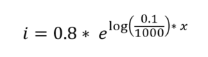
Here, i represents the intensity value to be calculated, and x represents the Euclidean distance to the nearest major road. I implemented this decay function to reflect both the presence of the road itself as well as the indirect effects of major roads, including light or noise pollution, which can exacerbate avoidance behaviors by organisms (Fahrig & Rytwinski, 2009).

I incorporated both the road density and road proximity datasets into the consolidated human footprint layer, resulting in a final 30-m human disturbance intensity surface. The maximum intensity value for a given cell among all three input datasets became the final value assigned to this surface.

Natural barriers to movement

To approximate the ease of movement across the landscape according to the presence and intensity of anthropogenic features, I converted the human modification surface into a conductance surface using a negative, linear transformation of intensity values. Conductance values were then multiplied (i.e., penalized) according to the presence of non-anthropogenic features and their ability to act as barriers to movement depending on the species group of interest (Table 5; Williamson et al., 2020). For generalist species, conductance values were multiplied by 0.8 for each pixel containing a non-grassland vegetation type; for specialist species, a conductance multiplier of 0.5 was instead applied to reflect a greater avoidance of non-preferred natural land cover types. The presence or absence of grassland land cover was ascertained using a combination of two datasets: a grasslands extent surface created in 2014 by the Grasslands Conservation Council of BC (GCC, 2014), and the 30-m North American land cover dataset. In regions where the grasslands extent surface identified grasslands and the land cover dataset did not, the former was assumed to be correct.

Using the 30-m North American land cover dataset, non-vegetated land cover types (barren, snow and ice, and water) were assigned a conductance multiplier of 0.5 to reflect the increased difficulty of traversing through structurally simple landscapes that are dissimilar to the preferred habitat type (Prevedello & Vieira, 2010). Conductance values were additionally multiplied by 0.8 if pixels exhibited a very high terrain ruggedness value. Large (>1km²) water bodies were automatically assigned a conductance value irrespective of other natural or anthropogenic features associated with a pixel: for high-mobility species, I applied a value of 0.5 to reflect the ability of large water bodies to act as moderate barrier to movement, whereas for low-mobility species, I instead used a value of 0.1 to reflect the ability of large water bodies to pose a much greater barrier to movement. The final 30-m conductance surfaces that were developed reflected overall landscape permeability for each of the four generic species groups.

3. Modeling connectivity

Model inputs

ConScape requires several inputs to model habitat functionality and proximity-weighted betweenness: the permeability of the landscape in terms of both its likelihood (A) and cost (C), and the quality of habitat as a source (q^s) and as a target (q^t). These inputs allow for greater flexibility and accuracy in instances where there is comprehensive data for the species of interest; however, ConScape also accepts simplified inputs when data is limited, or the analysis is not specific to any one particular species. Because my analysis lacked species-specific data and aimed to model connectivity for a broad range of species, I provided all inputs as a function of the conductance surfaces created previously (Table 6). Conductance was directly provided as movement likelihood, whereas movement cost was provided as a negatively log-transformed function of likelihood under the assumption that species movement is well-adapted to the environment. Habitat quality, both as a source and as a target, was provided as an exponential transformation of movement likelihood; this assumes that permeability is correlated with habitat quality (Prevedello & Vieira, 2010), but that regions of moderate movement likelihood (e.g., non-grasslands with low disturbance intensity) still represent relatively poor-quality habitat.

Movement behaviour and dispersal ability

By incorporating a randomized shortest paths (RSP) framework into its models, ConScape allows the user to control the randomness of movement using the parameter Ɵ: as Ɵ → 0, movement approaches a random walk, whereas at Ɵ → ∞, movement approaches a least-cost path. After testing a range of values, I decided to implement a Ɵ value of 1 to reflect some degree of exploratory movement away from optimal routes as organisms disperse throughout the landscape. ConScape also requires a scaling parameter, α, when exponentially transforming the distance between source and target pixels to proximity based on the movement capabilities of the species of interest. Proximity values can range from zero to one, where zero represents no ecological connectivity between pixels and one represents perfect ecological connectivity between pixels. I defined α as the maximum dispersal distances defined for each focal species group (Table 1) so that the proximity between source and target locations approaches zero as the maximum dispersal distance is exceeded.

Habitat functionality and proximity-weighted betweenness

After defining the required inputs and parameters, I ran ConScape’s habitat functionality and proximity-weighted betweenness functions individually for each species group. Because both processes are computationally intensive, I divided the study area into tiles and ran the analysis on each tile individually. Each tile spanned at least double the width and height of the maximum dispersal distance defined for each species group to prevent artificial barriers from being introduced; overlapping buffers surrounding each tile, each at least the size of the maximum dispersal distance of each species group, were also included to prevent the introduction of these barriers and to allow tiles to be subsequently merged (Ravary, 2024) . To further reduce the computational load and runtime to reasonable levels, I resampled the input surfaces to 300-m and 600-m resolutions for low-mobility and high-mobility groups, respectively. After running the analysis for each individual species group, I combined results by calculating mean habitat functionality and proximity-weighted betweenness values across all species groups for each pixel in the landscape, allowing me to identify shared regions of high connectivity value for a broad range of grassland-associated species.

Data Sources

The models incorporated in the Ecosystem Explorer leverage a diverse set of data, including Earth-Observation satellite imagery, climate data, LiDAR data (where available), provincial datasets, the Canadian Digital Elevation Model (CDEM) and field observations to predict future and characterize wetland and grassland distributions.

Please contact the following for more information about data sources:

• Wetlands extent predictive models including case study: Kristina Deenik | kdeenik [at] geodesicsolutions.net
• Grasslands connectivity models: Brittany Adams | brittany.adams1995 [at] gmail.com
• Grasslands extent predictive models (summer 2025 updates): Mathieu Bourbonnais | mathieu.bourbonnais [at] ubc.ca